Support Vector Machines? Separate data with largest possible margin!
Content:
- Definition
- Hard margin (data is linearly-separable)
- Soft margin (data is not linearly-separable)
- Kernel trick
- ‘C’ parameter
- \(\gamma\) parameter
- Strengths
- Weaknesses
- References
Definition
Support Vector Machines(SVMs for short), in the context of machine learning, are the ways to separate data between two (or more) categories. (The context here used in the supervised machine learning, one in which all the data examples are labeled with their correct categories). Basically an SVM model is representation of the examples as points in space, mapped so that the examples of the separate categories are divided by a clear gap(hyperplane) that is as wide as possible. New examples are then mapped into that same space and predicted to belong to a category based on the side of the hyperplane on which they fall. Below picture depicts the function of SVM in which the red line is the boundary which SVM tries to find:-
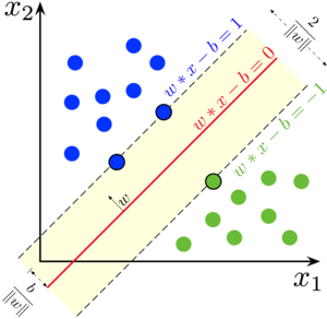
In machine learning the boundary that separates the examples of the different classes is termed as “Decision boundary”, which in context of SVM is known as a ‘hyperplane’. In next section we discuss the equation which is mentioned in the image.
The equation of the hyperplane is given by two parameters, a real-values vector \(w\) and input vector \(x\) and a real number \(b\) like this: \(w*x - b = 0\)
For the new input vector \(x\) the equation to predict the class will be given by: \(w*x - b = y\)
We want to find the maximum margin hyperplane that divides the group of points x for which \(y = 1\) from the group of points for which \(y = -1\) . A large margin contributes to the better generalization, that is how the model will work on the new examples in the future. To minimize that we minimize the Euclidean norm of the \(w\) denoted by \(\|w\|\) and given by
\[\ ||w|| = \sqrt \sum W ^2\]Hard margin (data is linearly-separable)
But why by minimizing the norm of w do we find the highest margin between two classes? Geometrically the equations \(wx-b = 1\) and \(wx-b = -1\) define two parallel hyperplanes. The distance between these hyperplanes is given by \(\frac{2}{\|w\|}\), so the smaller the norm \(||w||\), the larger the distance between these two hyperplanes. That was the mathematics of SVM.
Below is the small python example of the same:
from sklearn import svm
X = [[0, 0], [1, 1]]
y = [0, 1]
clf = svm.SVC()
clf.fit(X, y)
output:
SVC(C=1.0, cache_size=200, class_weight=None, coef0=0.0,
  decision_function_shape='ovr', degree=3, gamma='auto', kernel='rbf',
  max_iter=-1, probability=False, random_state=None, shrinking=True,
  tol=0.001, verbose=False)
After being fitted, the model can then be used to predict new values:
clf.predict([[2., 2.]])
output:
array([1])
Some properties of these support vectors can be found in members support_vectors_, support_ and n_support
# get support vectors
clf.support_vectors_
output:
array([[0., 0.],
       [1., 1.]])
get indices of support vectors
clf.support_
output:
array([0, 1])
get number of support vectors for each class
clf.n_support_
output:
array([1, 1])
Soft margin (data is not linearly-separable)
Additionally, for the data which is not linearly-separable, SVMs use another function called hinge loss function. It is given by: \(max(0, 1-y(wx - b))\)
for the data on the wrong side of the margin, the function’s value is proportional to the distance from the margin. So in that case we wish to minimize:
\[\bigg[ \frac{1}{n} \sum max(0, 1 - y(w * x - b))\bigg] + \lambda||w||^2\]Kernel trick
Kernels are the functions that taken a low-dimensional feature space and map it to a high-dimensional feature space in order to make the data linearly separable which previously was not. Calculate the solution into this high-dimensional space and get back to the previous dimensional space. The resultant separation is thus non-linear.
Kernels can be of the following types: -
- linear: \((x, x')\)
- polynomial: \((\gamma(x, x')+r)^d\). \(d\) is specified by keyword degree, \(r\) by \(coef0\)
- rbf: \(exp(-\gamma\|x - x'\|^2)\). \(\gamma\) is specified by keyword gamma, must be greater than \(0\)
- sigmoid: \(tanh(\gamma(x, x')+r)\) where \(r\) is specified by \(coef0\)
- custom
Below is the python example:
setting up a ‘linear kernel’
linear_svc = svm.SVC(kernel='linear')
linear_svc.kernel
output:
'linear'
setting up an ‘rbf kernel’
rbf_svc = svm.SVC(kernel='rbf')
rbf_svc.kernel
output:
'rbf'
setting up a ‘custom kernel’
import numpy as np
from sklearn import svm
def my_kernel(X, Y):
    return np.dot(X, Y.T)

clf = svm.SVC(kernel=my_kernel)
clf.kernel
output:
<function __main__.my_kernel(X, Y)>
‘C’ parameter of SVMs
The ‘C’ parameter controls the trade-off between smooth decision boundary and classifying training points correctly. A large ‘C’ values yields more training points correct and a lower ‘C’ values yields a smooth decision boundary.
\(\gamma\) parameter of SVMs
The gamma parameter defines how far the influence of a single training example reaches. A low value of gamma will cause the SVM to take farther data points into the account to create the decision boundary and high value for the closest data point.
Strengths of SVMs
- Effective in high dimensional spaces.
- Still effective in cases where number of dimensions is greater than the number of samples.
- Uses a subset of training points in the decision function (called support vectors), so it is also memory efficient.
- Versatile: different Kernel functions can be specified for the decision function. Common kernels are provided, but it is also possible to specify custom kernels.
Weaknesses of SVMs
- If the number of features is much greater than the number of samples, avoid over-fitting in choosing Kernel functions and regularization term is crucial.
- SVMs do not directly provide probability estimates, these are calculated using an expensive five-fold cross-validation (see Scores and probabilities, below).
Hope you enjoyed the post…