What makes the Deep Learning "Deep"? Multiple layers and backpropagation
Definition of a neural-network
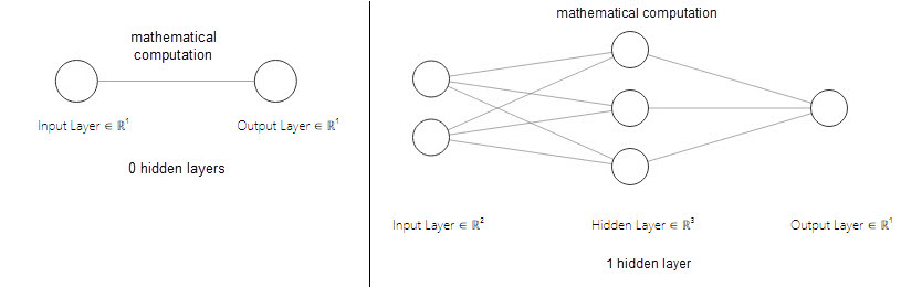
Besides the biological inspiration from human mind, the neural networks actually are the universal function approximators. They just compute a mathematical function. They take several inputs, process them through multiple neurons from 0 or more hidden layers and return the result using an output layer. Below image depicts the structure of a neural network with 0 and 1 hidden layer–
Building blocks of a neural-network
1. Perceptron : -
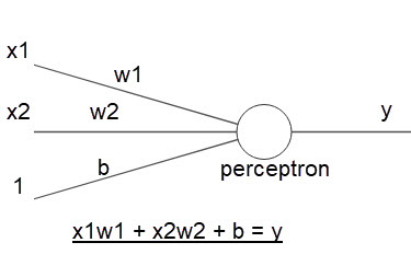
Perceptron is the basic unit of a neural-network. It can be understood as anything that takes input(s) and produces output(s). In the above picture x is supplied as an input into the perceptron (consider the round shaped object as a perceptron), it will perform the calculation and will give the result as y. The calculation can be functioned as anything. Similarly the form of the output can be functioned as anything. For example: suppose x has some value, the calculation we function as ‘multiplication with any number w’. The output we function as if the multiplication operation between x and w meets some threshold value t then output 1 otherwise output 0. Mathematically putting: { x * w = y; if y >= t output 1, otherwise 0}
2. Weights : -
Weights assign the importance to the perceptrons. So during calculation the neural-network treats the inputs more or less important in calculating the output. We just multiply each input with their respective weight values to make it more or less relevant to the output.
3. Biases : -
Bias defines the flexibility of perceptrons. It’s just a constant value which adds to the operation of input * weights.
The whole operation of the neural operation can we interpreted as the equation of a linear function: -
linear equation: y = mx + b
Below is the picture of neural-network depicting the building blocks: -
Multi Layer Perceptrons (MLP)
An MLP consists of the multiple hidden layers stacked between the input and the output layer. See the below picture having 2 hidden layers: -
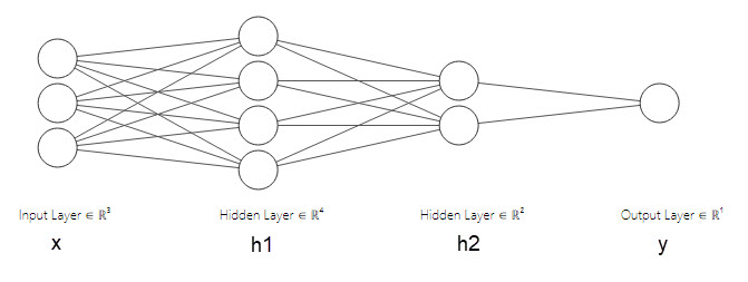
The notion is: every neuron in a single layer is connected with each of the neurons in its subsequent layer. i. e. in the above picture each of the 3 neurons in layer x will be connected with all the 4 neurons in h1 layer thus making total 3 x 4 = 12 connections, each of the 4 neurons in layer h1 will be connected with all the 2 neurons in h2 layer thus making total 4 x 4 = 16 connections and so on till the layers go on. From this stacking of the layers one-after-the-other only deep learning got the word deep in its name.
Activation Function
As we saw previously that the output of a perceptron comes from the sum of weighted inputs (x1w1+x2w2+b). That defines a linear function. However activations functions introduce $non-linear$ properties to our neural network. They help the neural-network to make sense of something really complicated and non-linear functional mappings between the inputs and the outputs. Their main purpose is to convert an input signal of a node in neural-network to an output signal. That output signal is used as a input in the next layer in the stack. There are several activation functions out there. Below are the 3 mostly used so far: -
- ReLU
- Sigmoid
- tanh
So to break it down what is the actual functioning of a neural-network is?
input times weight, add a bias, activate! input times weight, add a bias, activate! …
Backpropagation: enable learning
Till now we saw the process of computing the function through neural network by passing the outputs from one layer as the input to other subsequent layers by going forward in the direction. This is called forward-propagation. In the last layer(the output layer) we get the final output computed by the entire network. What’s next? Here we compare the outputs from the actual ones. That may or may not match. When they don’t match we take the difference between the both outputs - the actual ones and the computed ones. We want to reduce this error as much as we can.
So we backpropagate through the network. That is we go in backward direction layer by layer. And we compute the amount of error contributed by each layer into the entire amount of error. According to this individual error contributed by each layer we adjust the weights and biases so that in the next iteration of computation the error will be less. This weight and bias updating process going backward is known as “Back Propagation”. The process which involves in backpropagation to minimize the error is to determine the gradients (Derivatives) of each node w.r.t. the final output.
The adjustment in the weights and biases will be happening by either increasing them (moving into upward direction) or by decreasing them (moving into downward direction). We move the weights upward or downward based on whichever direction brings down the error the most. This process is of moving the weights into one of the appropriate directions, is known as gradient-descent.
Building our own Deep-Neural-network
The prerequisite is only the knowledge of basic python syntax.
import numpy as np
np.random.seed(3)
#Input array
X=np.array([[1,0,1,0],[1,0,1,1],[0,1,0,1]])

#Output
y=np.array([[1],[1],[0]])
#Sigmoid Function
def sigmoid (x):
    return 1/(1 + np.exp(-x))

#Derivative of Sigmoid Function
def sigmoid_derivatives(x):
    return x * (1 - x)
#Variable initialization
epoch=10001 #Setting training iterations
learning_rate=0.1 #Setting learning rate
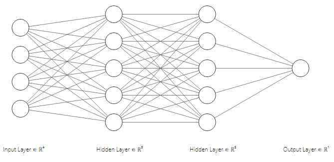
inputlayer_neurons = X.shape[1] #number of features in data set
hiddenlayer1_neurons = 5 #number of 1st hidden layer's neurons
hiddenlayer2_neurons = 5 #number of 2nd hidden layer's neurons
output_neurons = 1 #number of neurons at output layer
#weight and bias initialization
weights_input_to_hidden1 = np.random.normal(size=(inputlayer_neurons,hiddenlayer1_neurons))
bias_input_to_hidden1 =np.random.normal(size=(1,hiddenlayer1_neurons))

weights_hidden1_to_hidden2 = np.random.normal(size=(hiddenlayer1_neurons, hiddenlayer2_neurons))
bias_hidden1_to_hidden2 =np.random.normal(size=(1,hiddenlayer2_neurons))

weights_hidden2_to_output = np.random.normal(size=(hiddenlayer2_neurons,output_neurons))
bias_hidden2_to_output=np.random.normal(size=(1,output_neurons))
#Initial weights and biases
print(np.sum(weights_input_to_hidden1))
print(np.sum(weights_hidden1_to_hidden2))
print(np.sum(weights_hidden2_to_output))

print(np.sum(bias_input_to_hidden1))
print(np.sum(bias_hidden1_to_hidden2))
print(np.sum(bias_hidden2_to_output))
-1.80831494926
-12.1964091106
-4.6507139537
-0.691616944068
5.58110257009
1.04814751225
Below is the graphical representation of our neural network
for i in range(epoch):
    #Forward Propogation
    hidden_layer1_activations = sigmoid(np.dot(X, weights_input_to_hidden1) + bias_input_to_hidden1)
    hidden_layer2_activations = sigmoid(np.dot(hidden_layer1_activations, weights_hidden1_to_hidden2) + bias_hidden1_to_hidden2)
    output_layer_activations = sigmoid(np.dot(hidden_layer2_activations, weights_hidden2_to_output) + bias_hidden2_to_output)

    #Backpropagation

    #getting the error contribution by each layer
    #output to hidden2
    error_output_layer = y - output_layer_activations
    slope_output_layer = sigmoid_derivatives(output_layer_activations)
    delta_output_layer = error_output_layer * slope_output_layer

    #hidden2 to hidden1
    slope_hidden_layer2 = sigmoid_derivatives(hidden_layer2_activations)
    error_hidden_layer2 = delta_output_layer.dot(weights_hidden2_to_output.T)
    delta_hidden_layer2 = error_hidden_layer2 * slope_hidden_layer2

    #hidden1 to input
    slope_hidden_layer1 = sigmoid_derivatives(hidden_layer1_activations)
    error_hidden_layer1 = delta_hidden_layer2.dot(weights_hidden1_to_hidden2.T)
    delta_hidden_layer1 = error_hidden_layer1 * slope_hidden_layer1

    #weight and bias adjustments
    #output to hidden2
    weights_hidden2_to_output += hidden_layer2_activations.T.dot(delta_output_layer) * learning_rate
    bias_hidden2_to_output += np.sum(delta_output_layer, axis=0, keepdims=True) * learning_rate

    #hidden2 to hidden1
    weights_hidden1_to_hidden2 += hidden_layer1_activations.T.dot(delta_hidden_layer2) * learning_rate
    bias_hidden1_to_hidden2 += np.sum(delta_hidden_layer2, axis=0, keepdims=True) * learning_rate

    #hidden1 to input
    weights_input_to_hidden1 += X.T.dot(delta_hidden_layer1) * learning_rate
    bias_input_to_hidden1 += np.sum(delta_hidden_layer1, axis=0, keepdims=True) * True

    if i != 0 and i % 1000 == 0:
        print("error after {0} steps of training: {1}".format((i/1000*1000),np.sum(error_output_layer)))
error after 1000.0 steps of training: 0.05017865758179757
error after 2000.0 steps of training: 0.03385905514684301
error after 3000.0 steps of training: 0.02710604724361674
error after 4000.0 steps of training: 0.02320838959075526
error after 5000.0 steps of training: 0.020600783378227717
error after 6000.0 steps of training: 0.018702242763037086
error after 7000.0 steps of training: 0.017241741293459033
error after 8000.0 steps of training: 0.01607384469810294
error after 9000.0 steps of training: 0.015112688435244877
error after 10000.0 steps of training: 0.014303920134778207
Here we can see that after every 1000 iterations the error is coming down. That is what the learning is. Below are the changes in the weights from start till last iteration and the outputs actual and learnt.
Comparisons between initial weights and learnt weights, initial biases and learnt biases
| fromLayer-toLayer | Initial | Learnt |
|---|---|---|
| weights_input_to_hidden1 | -1.80831494926 | 0.734977377377 |
| weights_hidden1_to_hidden2 | -12.1964091106 | -19.7391252451 |
| weights_hidden2_to_output | -4.6507139537 | -8.00229057249 |
| bias_input_to_hidden1 | -0.691616944068 | -1.59037685196 |
| bias_hidden1_to_hidden2 | 5.58110257009 | 6.57941831296 |
| bias_hidden2_to_output | 1.04814751225 | 2.33347094143 |
#Learnt weights and biases
print(np.sum(weights_input_to_hidden1))
print(np.sum(weights_hidden1_to_hidden2))
print(np.sum(weights_hidden2_to_output))

print(np.sum(bias_input_to_hidden1))
print(np.sum(bias_hidden1_to_hidden2))
print(np.sum(bias_hidden2_to_output))
0.734977377377
-19.7391252451
-8.00229057249
-1.59037685196
6.57941831296
2.33347094143
Comparisons between actual outputs learnt outputs
| Actual | Learnt |
|---|---|
| 1 | 0.98575026 |
| 1 | 0.98088523 |
| 0 | 0.01906059 |
print(y)
print(output_layer_activations)