Regularize (L2, L1, Dropout) your neural network to prevent overfitting.
Underfitting and Overfitting - notion of Bias and Variance
The learning algorithms (supervised) learn a model from already provided data, we often call training data. The goal of the learning algorithm to learn a mapping function f between input variable X and output variable Y. The mapping function also called the target function as this is the function which the model tries to approximate. Throughout the iterative process of learning, the model keeps on trying to reduce the error between X and Y. Two things out of the many more can be taken into account to measure the error: -
- Bias
- Variance
Bias
Biases are the simplyfying assumptions made by a model to make the target function easier to learn. Though it helps the model to reach the target but a high bias(erroneous assumptions) can cause a model to miss the relevant relations between input features and target outputs. That is called underfitting.
Variance
Variance is an estimate of amount of change in the target function if different training data is used. Ideally we want the target function to not to change too much from one dataset to another. A high variance can cause a model to capture the random noise (unwanted information) from the data. That is called overfitting.
Choosing the right amount of bias and variance can be seen as a person trying to get the jeans of just perfect fit. The skinny jeans are good for the fit. But they are usually hard to come by. People neither want to take the jeans too skinny for their body(underfit) nor they want it to be too loose(overfitting). So a nominal size is to be selected that is just fine for them.
Let’s see the picture below to have a closer look on an underfitting, overfitting and just fine model.
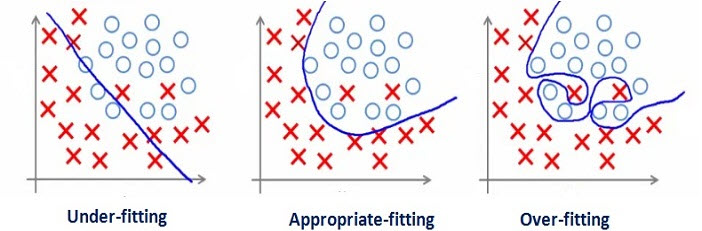
We can see from the picture above that in the first part the blue line of the model actually fails to separate the data-points well in different categories(ovals and crosses). That is an example of underfitting. The underfitting models performs poorly on the training data set as well as on the different datasets (validation or test sets from the same distribution or entirely others). While in the third part of the picture the model line is too well separating the both classes of the dataset. This model actually be called as overfitting as it models the information too well on the training data but fails to generalize it on the other datasets.
To solve the problem of high bias we should use a bigger model that would be able to get the relevant information out of the data and for the high variance problem more training data is one solution.
So now as we are aware of the fact overfitting, let’s see how we can prevent our model to overfit.
Preventing overfitting: Regularization
Regularization is a technique which makes slight modifications to the learning algorithm such that the model generalizes better. This in turn improves the model’s performance on the unseen data as well. The idea is to penalize the coefficients in the algorithm (weights in case of neural networks) by some amount.
Below are a few different techniques to apply regularization in deep learning.
- L2
- L1
- Dropout
L2 regularization
It is perhaps the most common form of regularization. It can be implemented by penalizing the squared magnitude of all parameters directly in the objective. That is, for every weight \(W\) in the network, we add the term \(\frac{1}{2} \lambda W^2\) to the objective, where \(\lambda\) is the regularization strength. It is common to see the factor of \(\frac{1}{2}\) in front because then the gradient of this term with respect to the parameter \(W\) is simply \(\lambda W\) instead of \(2 \lambda W\). The L2 regularization has the intuitive interpretation of heavily penalizing peaky weight vectors and preferring diffuse weight vectors. As we discussed in the Linear Classification section, due to multiplicative interactions between weights and inputs this has the appealing property of encouraging the network to use all of its inputs a little rather than some of its inputs a lot. Lastly, notice that during gradient descent parameter update, using the L2 regularization ultimately means that every weight is decayed linearly: \(W += - \lambda * W\) towards zero.
Performing L2 regularization
\[Cost \ function = Loss \ + \ \frac{\lambda}{2m} \ * \ \sum \mid W \mid^2\]Here, lambda is the regularization parameter. It is the hyperparameter whose value is optimized for better results. L2 regularization is also known as weight decay as it forces the weights to decay towards zero (but not exactly zero).
L1 Regularization
It is another relatively common form of regularization, where for each weight \(W\) we add the term \(\lambda \mid W \mid\) to the objective. The L1 regularization has the intriguing property that it leads the weight vectors to become sparse during optimization (i.e. very close to exactly zero). In other words, neurons with L1 regularization end up using only a sparse subset of their most important inputs and become nearly invariant to the “noisy” inputs. In comparison, final weight vectors from L2 regularization are usually diffuse, small numbers. In practice, if you are not concerned with explicit feature selection, L2 regularization can be expected to give superior performance over L1.
Performing L1 regularization
\[Cost \ function = Loss \ + \ \frac{\lambda}{m} \ * \ \sum \mid W \mid\]In this, we penalize the absolute value of the weights. Unlike L2, the weights may be reduced to zero here. Hence, it is very useful when we are trying to compress our model. Otherwise, we usually prefer L2 over it.
Dropout
According to Wikipedia —
The term “dropout” refers to dropping out units (both hidden and visible) in a neural network.
Simply put, dropout refers to ignoring units (i.e. neurons) during the training phase of certain set of neurons which is chosen at random. By “ignoring”, it means these units are not considered during a particular forward or backward pass. That is at each training stage, individual nodes are either dropped out of the net with probability \(1-p\) or kept with probability \(p\), so that a reduced network is left; incoming and outgoing edges to a dropped-out node are also removed.
See the below picture to understand it better: -
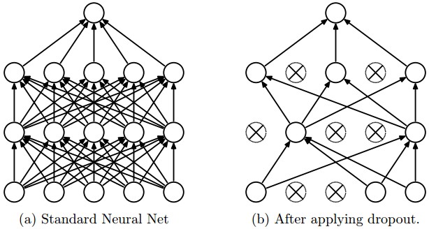
Figure taken from the Dropout paper that illustrates the idea.
Below is the code to install dropout in any network: -
import numpy as np
np.random.seed(3)
X = np.array([ [0,0,1],[0,1,1],[1,0,1],[1,1,1] ])
y = np.array([[0,1,1,0]]).T
learning_rate,hidden_dim,dropout_percent,do_dropout = (0.5,4,0.2,True)
synapse_0 = 2*np.random.random((3,hidden_dim)) - 1
synapse_1 = 2*np.random.random((hidden_dim,1)) - 1
for j in range(60000):
    layer_1 = (1/(1+np.exp(-(np.dot(X,synapse_0)))))
    if(do_dropout):
        d1 = np.random.randn(len(X),hidden_dim)    # Step 1: initialize matrix d1 = np.random.rand(..., ...)
        d1 = (d1 > dropout_percent)                # Step 2: convert entries of d1 to 0 or 1 (using keep_prob as the threshold)
        layer_1 = layer_1 * d1                     # Step 3: shut down some neurons of layer_1
        layer_1 = layer_1 / dropout_percent        # Step 4: scale the value of neurons that haven't been shut down

    layer_2 = 1/(1+np.exp(-(np.dot(layer_1,synapse_1))))
    layer_2_delta = (layer_2 - y)*(layer_2*(1-layer_2))
    layer_1_delta = layer_2_delta.dot(synapse_1.T) * (layer_1 * (1-layer_1))
    synapse_1 -= (learning_rate * layer_1.T.dot(layer_2_delta))
    synapse_0 -= (learning_rate * X.T.dot(layer_1_delta))
Hope you enjoyed the post…